> ## Documentation Index
> Fetch the complete documentation index at: https://docs.nikaplanet.com/llms.txt
> Use this file to discover all available pages before exploring further.
# Raster Layer Styling
> Customize raster layer visualization with band selection, color modes, range adjustments, and spectral indices
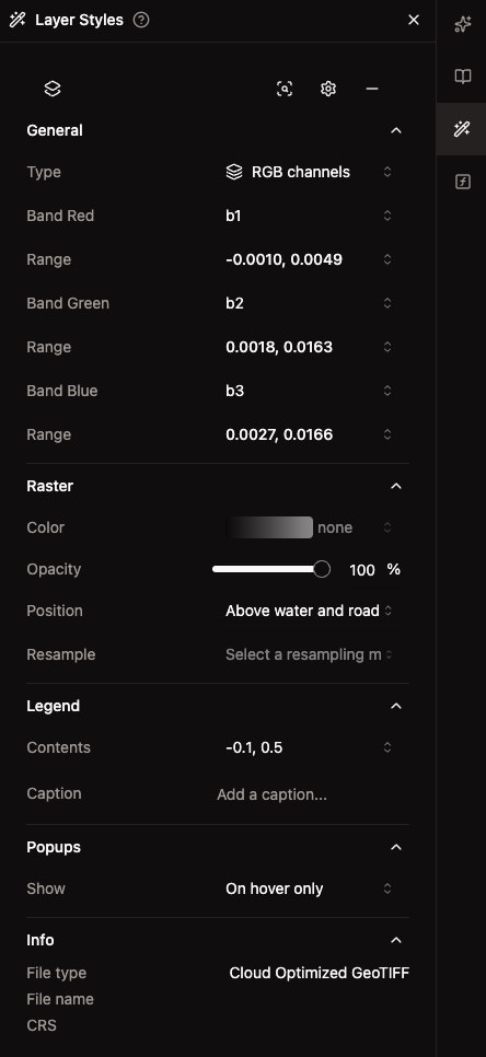
Customize how your raster layers appear on the map using the Layer Styles panel. Control visualization types, band selection, color mapping, and data ranges to effectively display your raster data.
 ## How to Style Raster Layers
### Access Styling Panel
1. **Click on a raster layer** in the layers panel to select it
2. The **styling panel opens** on the side with all raster customization options
3. Use the **header buttons** to zoom to the layer, access layer settings (rename, remove, etc.), or unselect the layer
### Available Styling Sections
#### **General Section**
* **Type**: Choose visualization method — Single Channel, RGB Channels, Raster Algebra, or Hillshade
* **Band Selection**: Select which bands to display (options change based on type)
* **Range**: Set data range for each band using absolute values or percentiles
#### **Raster Section**
* **Color Mode** (Single Channel only): Choose between Named Colormap, Classify, or Unique Values
* **Color**: Select a color map from grouped presets, or configure custom classification stops
* **Clip** (Google Earth Engine layers only): Clip the raster to a polygon vector layer on the map
* **Opacity**: Adjust layer transparency (0–100%) with a slider and numeric input
* **Position**: Control layer stacking order
* **Resample**: Select resampling method for zoom levels
#### **Legend Section**
* **Show**: Toggle legend visibility on or off
* **Caption**: Add descriptive text for the layer legend
#### **Popups Section**
* **Show**: Configure when popup information appears (Hover Only)
#### **Info Section**
* **File type**: Shows raster format — Cloud Optimized GeoTIFF or GeoTIFF (with a warning if not cloud-optimized)
* **File name**: Display file name
* **CRS**: Show coordinate reference system
## Visualization Types
## How to Style Raster Layers
### Access Styling Panel
1. **Click on a raster layer** in the layers panel to select it
2. The **styling panel opens** on the side with all raster customization options
3. Use the **header buttons** to zoom to the layer, access layer settings (rename, remove, etc.), or unselect the layer
### Available Styling Sections
#### **General Section**
* **Type**: Choose visualization method — Single Channel, RGB Channels, Raster Algebra, or Hillshade
* **Band Selection**: Select which bands to display (options change based on type)
* **Range**: Set data range for each band using absolute values or percentiles
#### **Raster Section**
* **Color Mode** (Single Channel only): Choose between Named Colormap, Classify, or Unique Values
* **Color**: Select a color map from grouped presets, or configure custom classification stops
* **Clip** (Google Earth Engine layers only): Clip the raster to a polygon vector layer on the map
* **Opacity**: Adjust layer transparency (0–100%) with a slider and numeric input
* **Position**: Control layer stacking order
* **Resample**: Select resampling method for zoom levels
#### **Legend Section**
* **Show**: Toggle legend visibility on or off
* **Caption**: Add descriptive text for the layer legend
#### **Popups Section**
* **Show**: Configure when popup information appears (Hover Only)
#### **Info Section**
* **File type**: Shows raster format — Cloud Optimized GeoTIFF or GeoTIFF (with a warning if not cloud-optimized)
* **File name**: Display file name
* **CRS**: Show coordinate reference system
## Visualization Types
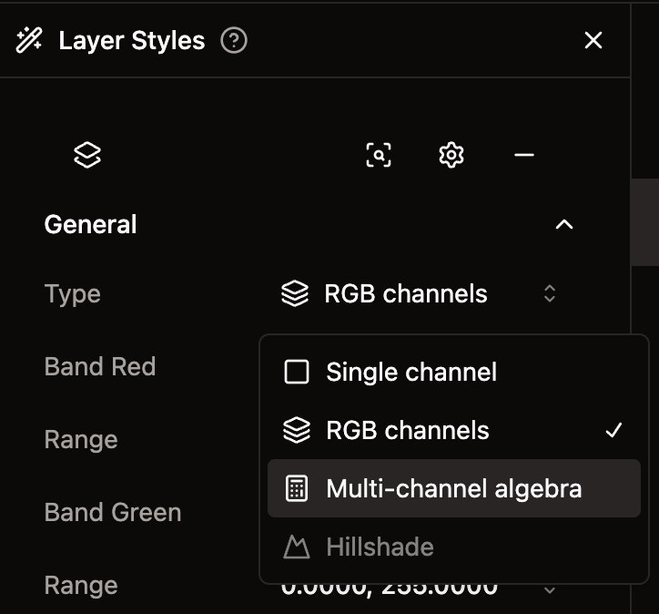 ### Single Channel
* **Display one band** at a time
* **Choose band**: Select from any available band in the dataset
* **Set range**: Adjust min/max values for the selected band
* **Apply color mode**: Use Named Colormaps, Classify, or Unique Values
### RGB Channels
Available when the raster has more than one band.
* **Display three bands** mapped to red, green, and blue channels
* **Band Red / Green / Blue**: Select which band maps to each channel
* **Individual ranges**: Set min/max or percentile values independently for each channel
### Raster Algebra
Available for non-GEE rasters with more than one band. Compute spectral indices from band math.
* **Select an expression**: Choose from built-in spectral indices
* **Map bands**: Assign which dataset bands correspond to each variable in the formula
* **Set range**: Adjust display range for the computed result
#### Built-in Spectral Indices
| Index | Formula | Description |
| --------- | ----------------------------------------- | ---------------------------------------------------- |
| **NDVI** | `(NIR-R)/(NIR+R)` | Vegetation health and density |
| **EVI** | `2.5*((NIR-R)/(NIR+6*R-7.5*B+1))` | Enhanced vegetation, high-biomass sensitivity |
| **SAVI** | `((NIR-R)/(NIR+R+0.5))*(1.5)` | Soil-adjusted vegetation index |
| **NDWI** | `(G-NIR)/(G+NIR)` | Water body detection |
| **NBR** | `(NIR-SWIR)/(NIR+SWIR)` | Burn area and severity |
| **NDRE** | `(NIR-RedEdge)/(NIR+RedEdge)` | Chlorophyll content for precision agriculture |
| **GNDVI** | `(NIR-G)/(NIR+G)` | Chlorophyll concentration (more sensitive than NDVI) |
| **NDBI** | `(SWIR-NIR)/(SWIR+NIR)` | Urban areas and bare soil |
| **NDMI** | `(NIR-SWIR)/(NIR+SWIR)` | Vegetation water content |
| **ARVI** | `(NIR-(2*R-B))/(NIR+(2*R-B))` | Atmospherically resistant vegetation |
| **BSI** | `((SWIR+R)-(NIR+B))/((SWIR+R)+(NIR+B))` | Bare soil detection |
| **MSAVI** | `(2*NIR+1-sqrt((2*NIR+1)^2-8*(NIR-R)))/2` | Modified soil-adjusted vegetation |
| **BAI** | `1/((0.1-R)^2+(0.06-NIR)^2)` | Post-fire burn area emphasis |
| **GLI** | `(2*G-R-B)/(2*G+R+B)` | Green leaf fraction estimation |
| **CIG** | `(NIR/G)-1` | Leaf chlorophyll content |
### Hillshade
* **Select a band** for terrain shading (currently in preview)
## Band Range Adjustment
### Single Channel
* **Display one band** at a time
* **Choose band**: Select from any available band in the dataset
* **Set range**: Adjust min/max values for the selected band
* **Apply color mode**: Use Named Colormaps, Classify, or Unique Values
### RGB Channels
Available when the raster has more than one band.
* **Display three bands** mapped to red, green, and blue channels
* **Band Red / Green / Blue**: Select which band maps to each channel
* **Individual ranges**: Set min/max or percentile values independently for each channel
### Raster Algebra
Available for non-GEE rasters with more than one band. Compute spectral indices from band math.
* **Select an expression**: Choose from built-in spectral indices
* **Map bands**: Assign which dataset bands correspond to each variable in the formula
* **Set range**: Adjust display range for the computed result
#### Built-in Spectral Indices
| Index | Formula | Description |
| --------- | ----------------------------------------- | ---------------------------------------------------- |
| **NDVI** | `(NIR-R)/(NIR+R)` | Vegetation health and density |
| **EVI** | `2.5*((NIR-R)/(NIR+6*R-7.5*B+1))` | Enhanced vegetation, high-biomass sensitivity |
| **SAVI** | `((NIR-R)/(NIR+R+0.5))*(1.5)` | Soil-adjusted vegetation index |
| **NDWI** | `(G-NIR)/(G+NIR)` | Water body detection |
| **NBR** | `(NIR-SWIR)/(NIR+SWIR)` | Burn area and severity |
| **NDRE** | `(NIR-RedEdge)/(NIR+RedEdge)` | Chlorophyll content for precision agriculture |
| **GNDVI** | `(NIR-G)/(NIR+G)` | Chlorophyll concentration (more sensitive than NDVI) |
| **NDBI** | `(SWIR-NIR)/(SWIR+NIR)` | Urban areas and bare soil |
| **NDMI** | `(NIR-SWIR)/(NIR+SWIR)` | Vegetation water content |
| **ARVI** | `(NIR-(2*R-B))/(NIR+(2*R-B))` | Atmospherically resistant vegetation |
| **BSI** | `((SWIR+R)-(NIR+B))/((SWIR+R)+(NIR+B))` | Bare soil detection |
| **MSAVI** | `(2*NIR+1-sqrt((2*NIR+1)^2-8*(NIR-R)))/2` | Modified soil-adjusted vegetation |
| **BAI** | `1/((0.1-R)^2+(0.06-NIR)^2)` | Post-fire burn area emphasis |
| **GLI** | `(2*G-R-B)/(2*G+R+B)` | Green leaf fraction estimation |
| **CIG** | `(NIR/G)-1` | Leaf chlorophyll content |
### Hillshade
* **Select a band** for terrain shading (currently in preview)
## Band Range Adjustment
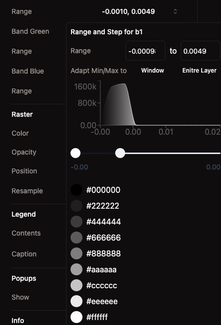 Click the **Range** button next to any band to open the range popover with a histogram and controls.
### Range Mode
* **Absolute**: Set explicit min and max values for the band
* **Percentile**: Set a low and high percentile (e.g., p2–p98) to clip outliers automatically
### Adjust Min/Max Values
1. **Open the range popover** by clicking the range display
2. **Choose a mode** — Absolute or Percentile
3. **Enter values** directly or **drag the histogram sliders** to set the range
4. **See real-time updates** on the map
### Adapt Min/Max To
* **Window**: Recalculate statistics based on the current map viewport
* **Entire Layer**: Reset to the full data range across the entire dataset
When adapted to a window, the range button shows a visual indicator. Click **Entire Layer** to reset.
### Histogram Display
* **Data distribution**: See how pixel values are spread across the band
* **Draggable range sliders**: Adjust min/max directly on the histogram
* **Color gradient preview**: The histogram reflects the currently applied color map
## Color Modes
Click the **Range** button next to any band to open the range popover with a histogram and controls.
### Range Mode
* **Absolute**: Set explicit min and max values for the band
* **Percentile**: Set a low and high percentile (e.g., p2–p98) to clip outliers automatically
### Adjust Min/Max Values
1. **Open the range popover** by clicking the range display
2. **Choose a mode** — Absolute or Percentile
3. **Enter values** directly or **drag the histogram sliders** to set the range
4. **See real-time updates** on the map
### Adapt Min/Max To
* **Window**: Recalculate statistics based on the current map viewport
* **Entire Layer**: Reset to the full data range across the entire dataset
When adapted to a window, the range button shows a visual indicator. Click **Entire Layer** to reset.
### Histogram Display
* **Data distribution**: See how pixel values are spread across the band
* **Draggable range sliders**: Adjust min/max directly on the histogram
* **Color gradient preview**: The histogram reflects the currently applied color map
## Color Modes
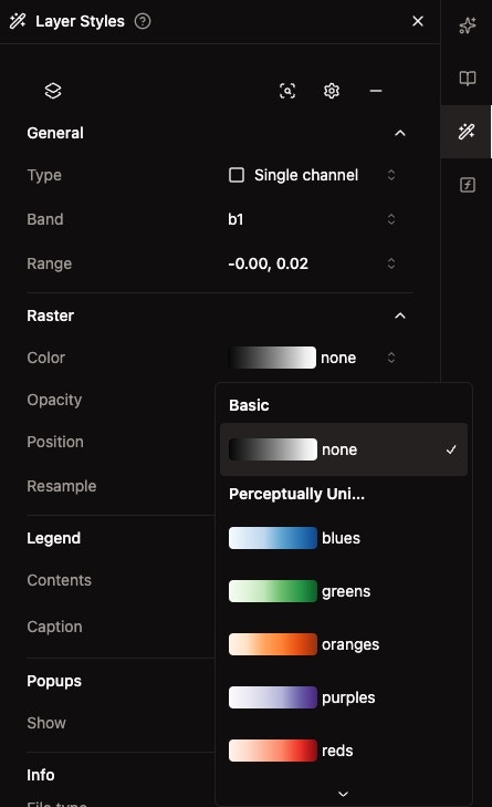 Color modes are available when using **Single Channel** visualization. RGB Channels always display the raw band values as red, green, and blue.
### Named Colormap
Select from a library of predefined color maps, organized by category:
| Category | Color Maps |
| ----------------------------------- | ------------------------------------------------------------------------------ |
| **Basic** | None (grayscale) |
| **Perceptually Uniform Sequential** | Blues, Greens, Oranges, Purples, Reds |
| **Sequential** | Viridis, Plasma, Inferno, Magma, Cividis |
| **Sequential 2** | BuGn, BuPu, GnBu, OrRd, PuBu, PuBuGn, PuRd, RdPu, YlGn, YlGnBu, YlOrBr, YlOrRd |
| **Diverging** | BrBG, PRGn, PiYG, PuOr, RdBu, RdGy, RdYlBu, RdYlGn, Spectral |
| **Cyclic** | Twilight, Twilight Shifted |
| **Qualitative** | Accent, Dark2, Paired, Pastel1, Pastel2, Set1, Set2, Set3 |
| **Miscellaneous** | Gist Earth, Terrain, Ocean, Jet, Rainbow, Cubehelix, and more |
Each color map shows a **gradient preview** in the dropdown so you can see the colors before applying.
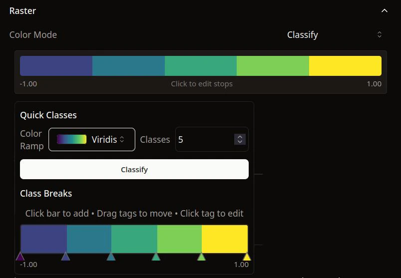
### Classify
Group pixel values into discrete classes with custom color stops.
* **Preset ramp**: Choose a starting color ramp
* **Number of classes**: Set how many bins to divide the data into (default: 5)
* **Apply**: Generate evenly spaced class breaks from the preset
* **Edit individual stops**: Adjust break values and colors for each class
Color modes are available when using **Single Channel** visualization. RGB Channels always display the raw band values as red, green, and blue.
### Named Colormap
Select from a library of predefined color maps, organized by category:
| Category | Color Maps |
| ----------------------------------- | ------------------------------------------------------------------------------ |
| **Basic** | None (grayscale) |
| **Perceptually Uniform Sequential** | Blues, Greens, Oranges, Purples, Reds |
| **Sequential** | Viridis, Plasma, Inferno, Magma, Cividis |
| **Sequential 2** | BuGn, BuPu, GnBu, OrRd, PuBu, PuBuGn, PuRd, RdPu, YlGn, YlGnBu, YlOrBr, YlOrRd |
| **Diverging** | BrBG, PRGn, PiYG, PuOr, RdBu, RdGy, RdYlBu, RdYlGn, Spectral |
| **Cyclic** | Twilight, Twilight Shifted |
| **Qualitative** | Accent, Dark2, Paired, Pastel1, Pastel2, Set1, Set2, Set3 |
| **Miscellaneous** | Gist Earth, Terrain, Ocean, Jet, Rainbow, Cubehelix, and more |
Each color map shows a **gradient preview** in the dropdown so you can see the colors before applying.
### Classify
Group pixel values into discrete classes with custom color stops.
* **Preset ramp**: Choose a starting color ramp
* **Number of classes**: Set how many bins to divide the data into (default: 5)
* **Apply**: Generate evenly spaced class breaks from the preset
* **Edit individual stops**: Adjust break values and colors for each class
 ### Unique Values
Available when all pixel values in the band are integers (up to 100 unique values).
* **Preset ramp**: Apply a color ramp across all unique values
* **Edit individual colors**: Click any color swatch to customize
* **Labels**: Add descriptive labels to each unique value for the legend
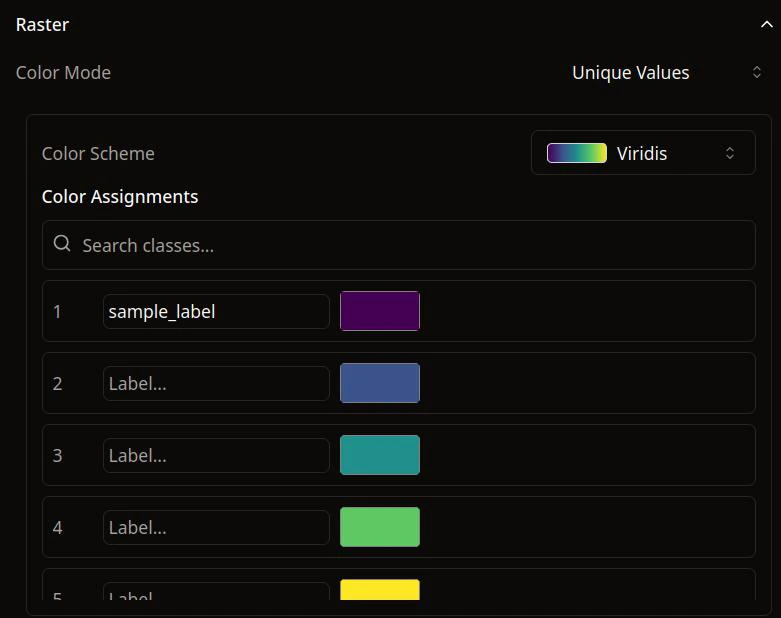
### Unique Values
Available when all pixel values in the band are integers (up to 100 unique values).
* **Preset ramp**: Apply a color ramp across all unique values
* **Edit individual colors**: Click any color swatch to customize
* **Labels**: Add descriptive labels to each unique value for the legend
 ## Resampling Methods
Control how pixel values are interpolated when zooming. Available methods:
* **Nearest**: No interpolation, preserves original values
* **Bilinear**: Linear interpolation between 4 nearest pixels
* **Cubic**: Cubic interpolation for smoother results
* **Cubic Spline**: Spline-based cubic interpolation
* **Lanczos**: High-quality resampling with Lanczos windowing
* **Average**: Average of contributing pixels
* **Mode**: Most common value among contributing pixels
* **Gauss**: Gaussian-weighted interpolation
* **RMS**: Root mean square of contributing pixels
## Auto-Save Feature
All styling changes are **automatically saved** for future sessions:
* **Settings persist** when you close and reopen the map
* **No manual saving** required
* **Consistent appearance** across sessions
* **Team collaboration** benefits from saved settings
## Best Practices
### Choose Appropriate Visualization
* **Single Channel**: For analyzing individual bands with color mapping
* **RGB Channels**: For natural color or false color composites
* **Raster Algebra**: For computing spectral indices like NDVI, NDWI, or custom band math
### Set Optimal Ranges
* **Use percentile mode** (e.g., p2–p98) to handle outliers without manual tuning
* **Use the histogram** to understand data distribution before setting ranges
* **Adapt to Window** to focus on the area you're currently viewing
### Select Suitable Color Modes
* **Named Colormap**: Best for continuous data — choose sequential for one-directional data (elevation, temperature) or diverging for data with a meaningful midpoint
* **Classify**: Best for categorizing continuous data into meaningful groups
* **Unique Values**: Best for categorical/integer rasters like land cover or classification results
## Next Steps
* **Add More Raster Layers**: Combine multiple raster datasets
* **Create Composites**: Build custom band combinations with Raster Algebra
* **Publish Your Map**: Share your styled raster layers
## Resampling Methods
Control how pixel values are interpolated when zooming. Available methods:
* **Nearest**: No interpolation, preserves original values
* **Bilinear**: Linear interpolation between 4 nearest pixels
* **Cubic**: Cubic interpolation for smoother results
* **Cubic Spline**: Spline-based cubic interpolation
* **Lanczos**: High-quality resampling with Lanczos windowing
* **Average**: Average of contributing pixels
* **Mode**: Most common value among contributing pixels
* **Gauss**: Gaussian-weighted interpolation
* **RMS**: Root mean square of contributing pixels
## Auto-Save Feature
All styling changes are **automatically saved** for future sessions:
* **Settings persist** when you close and reopen the map
* **No manual saving** required
* **Consistent appearance** across sessions
* **Team collaboration** benefits from saved settings
## Best Practices
### Choose Appropriate Visualization
* **Single Channel**: For analyzing individual bands with color mapping
* **RGB Channels**: For natural color or false color composites
* **Raster Algebra**: For computing spectral indices like NDVI, NDWI, or custom band math
### Set Optimal Ranges
* **Use percentile mode** (e.g., p2–p98) to handle outliers without manual tuning
* **Use the histogram** to understand data distribution before setting ranges
* **Adapt to Window** to focus on the area you're currently viewing
### Select Suitable Color Modes
* **Named Colormap**: Best for continuous data — choose sequential for one-directional data (elevation, temperature) or diverging for data with a meaningful midpoint
* **Classify**: Best for categorizing continuous data into meaningful groups
* **Unique Values**: Best for categorical/integer rasters like land cover or classification results
## Next Steps
* **Add More Raster Layers**: Combine multiple raster datasets
* **Create Composites**: Build custom band combinations with Raster Algebra
* **Publish Your Map**: Share your styled raster layers