 ## Mineral and Vegetation Index Calculation from Satellite Imagery
This Python script is designed to process GeoTIFF files, which are a common format for satellite and aerial imagery. The script calculates a series of remote sensing indices—specifically, mineral and vegetation indices—using different band combinations of the input imagery. It performs calculations like those for Ferrous Iron, Iron Oxide, Clay Minerals, Hematite, Gossan Minerals, Ferric Iron, NDVI (Normalized Difference Vegetation Index), Iron Oxide NIR, and Mineral Alteration NIR. The script then saves the calculated index values as new GeoTIFF files and generates two types of visualizations for each index: one showing the full range of values and another highlighting areas with high concentrations (above the 95th percentile). This process is useful for geological and environmental remote sensing applications, such as identifying potential mineral deposits or assessing vegetation health.
## Libraries Used
* **numpy**: Used for efficient numerical operations and array manipulation, which is essential for performing calculations on the image data
* **rasterio**: A key library for reading and writing geospatial raster data. It handles the I/O of GeoTIFF files, including their crucial metadata like coordinate reference systems and transformations
* **matplotlib.pyplot**: Used for creating static, interactive, and animated visualizations of the index results
* **os**: Provides a way to interact with the operating system, allowing the script to manage file paths and create directories
* **pathlib**: An object-oriented filesystem path library used for handling file paths more cleanly and cross-platform
## Input and Output Datasets
### Input Dataset
* One or more GeoTIFF (.tif or .tiff) files containing multi-band satellite imagery
* The script is designed to read these files from the specified input\_dir (/data/COPERNICUS/)
* The band numbers b1, b2, b3, etc., in the expressions correspond to the bands in the input TIFF file
### Output Datasets
For each input TIFF file, the script creates a new directory within the output\_dir (/data/Australia\_rare\_earth\_mine\_output/).
**Two GeoTIFF files are generated for each calculated index:**
* **{index_name}.tif**: A GeoTIFF file containing the calculated index values for the full range of data
* **{index_name}\_HighConcentration.tif**: A GeoTIFF file containing only the top 5% of index values, with the rest of the data set to a "no data" value (NaN). This highlights high-concentration areas
**One PNG visualization file is generated for each index:**
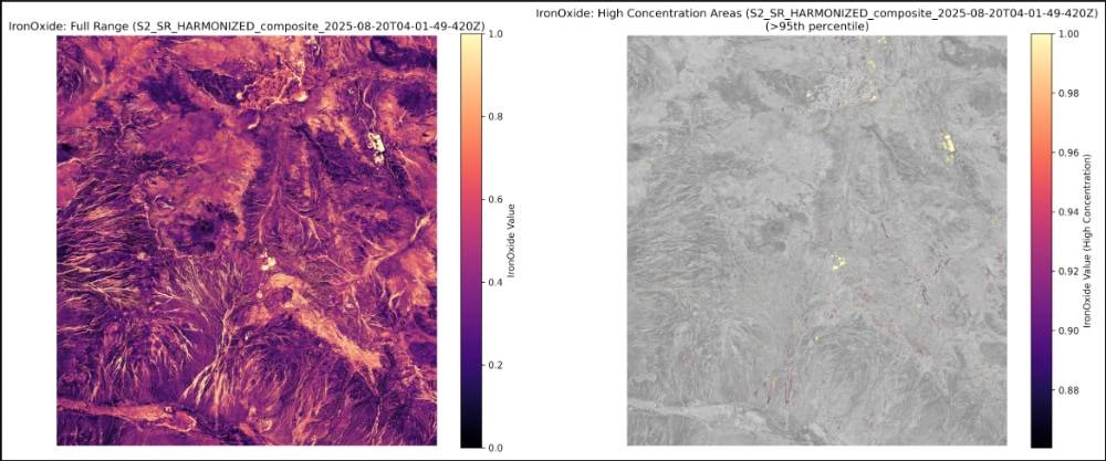
* **{index_name}\_visualization.png**: A single image file with two subplots: one showing the full-range index and another showing the high-concentration areas on a transparent background for easy identification
## Step-by-Step Implementation
### STEP-1: Sample Area Selection
The mine near Lenister area in Australia is taken as a sample using the geojson provided.
**Upload or create a new vector BBOX using DRAW function tab in Nika Map**
**Use data catalog to download the AOI as shown below**
The output is saved in `data/COPERNICUS`
### STEP-2: Code Execution
Run the code below:
Output saved in `/data/Australia_rare_earth_mine_output/S2_SR_HARMONIZED_composite_2025-08-20T04-01-49-420Z/`
**For each mineral profile:**
* The corresponding single channel TIF image is formed
* A second TIF image highlighting the highest concentration more than 95% percentile is saved separately (example: `ClayMineral_High_concentration.tif`)
**To make it more appealing:**
* Change the raster color to red using raster settings color
* A PNG image showing the scale of intensity is saved for each mineral component
***
## Mineral and Vegetation Index Calculation from Satellite Imagery
This Python script is designed to process GeoTIFF files, which are a common format for satellite and aerial imagery. The script calculates a series of remote sensing indices—specifically, mineral and vegetation indices—using different band combinations of the input imagery. It performs calculations like those for Ferrous Iron, Iron Oxide, Clay Minerals, Hematite, Gossan Minerals, Ferric Iron, NDVI (Normalized Difference Vegetation Index), Iron Oxide NIR, and Mineral Alteration NIR. The script then saves the calculated index values as new GeoTIFF files and generates two types of visualizations for each index: one showing the full range of values and another highlighting areas with high concentrations (above the 95th percentile). This process is useful for geological and environmental remote sensing applications, such as identifying potential mineral deposits or assessing vegetation health.
## Libraries Used
* **numpy**: Used for efficient numerical operations and array manipulation, which is essential for performing calculations on the image data
* **rasterio**: A key library for reading and writing geospatial raster data. It handles the I/O of GeoTIFF files, including their crucial metadata like coordinate reference systems and transformations
* **matplotlib.pyplot**: Used for creating static, interactive, and animated visualizations of the index results
* **os**: Provides a way to interact with the operating system, allowing the script to manage file paths and create directories
* **pathlib**: An object-oriented filesystem path library used for handling file paths more cleanly and cross-platform
## Input and Output Datasets
### Input Dataset
* One or more GeoTIFF (.tif or .tiff) files containing multi-band satellite imagery
* The script is designed to read these files from the specified input\_dir (/data/COPERNICUS/)
* The band numbers b1, b2, b3, etc., in the expressions correspond to the bands in the input TIFF file
### Output Datasets
For each input TIFF file, the script creates a new directory within the output\_dir (/data/Australia\_rare\_earth\_mine\_output/).
**Two GeoTIFF files are generated for each calculated index:**
* **{index_name}.tif**: A GeoTIFF file containing the calculated index values for the full range of data
* **{index_name}\_HighConcentration.tif**: A GeoTIFF file containing only the top 5% of index values, with the rest of the data set to a "no data" value (NaN). This highlights high-concentration areas
**One PNG visualization file is generated for each index:**
* **{index_name}\_visualization.png**: A single image file with two subplots: one showing the full-range index and another showing the high-concentration areas on a transparent background for easy identification
## Step-by-Step Implementation
### STEP-1: Sample Area Selection
The mine near Lenister area in Australia is taken as a sample using the geojson provided.
**Upload or create a new vector BBOX using DRAW function tab in Nika Map**
**Use data catalog to download the AOI as shown below**
The output is saved in `data/COPERNICUS`
### STEP-2: Code Execution
Run the code below:
Output saved in `/data/Australia_rare_earth_mine_output/S2_SR_HARMONIZED_composite_2025-08-20T04-01-49-420Z/`
**For each mineral profile:**
* The corresponding single channel TIF image is formed
* A second TIF image highlighting the highest concentration more than 95% percentile is saved separately (example: `ClayMineral_High_concentration.tif`)
**To make it more appealing:**
* Change the raster color to red using raster settings color
* A PNG image showing the scale of intensity is saved for each mineral component
***
Access the complete code, step-by-step instructions, and interactive notebook in Nika Hub.
View Full Solution →