> ## Documentation Index
> Fetch the complete documentation index at: https://docs.nikaplanet.com/llms.txt
> Use this file to discover all available pages before exploring further.

# River Corridor Urbanisation

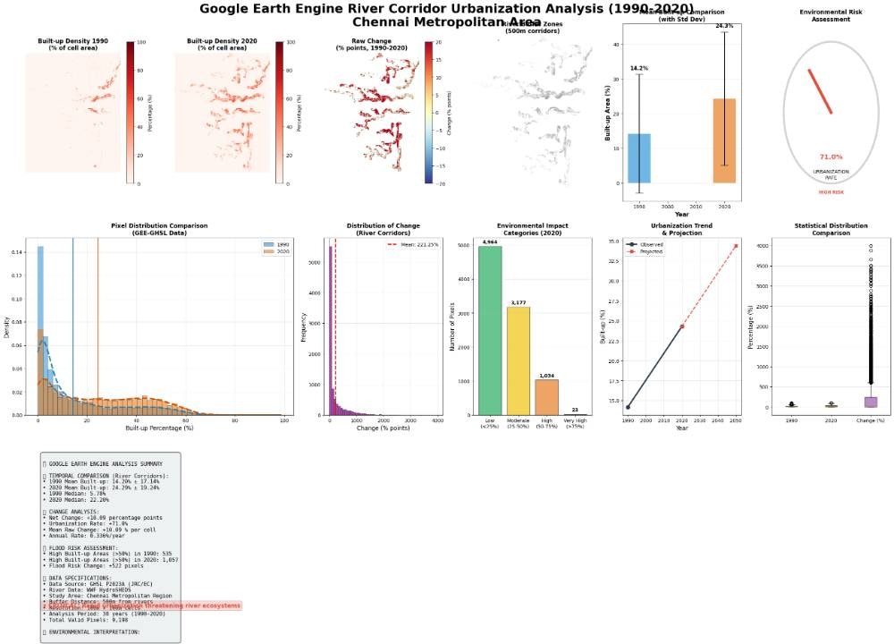
> Multi-temporal geospatial analysis with buffer-based proximity assessment to quantify urban encroachment patterns within river corridors

# River Corridor Urbanisation

<img src="https://mintcdn.com/nika/KF-c86_3b0KWdTjW/industrial-solutions/river-corridor-urbanisation.jpeg?fit=max&auto=format&n=KF-c86_3b0KWdTjW&q=85&s=8f91a021842c90f99efd3ff65593b1e2" alt="River Corridor Urbanisation" width="1000" height="720" data-path="industrial-solutions/river-corridor-urbanisation.jpeg" />

## Methodology

The analysis employs multi-temporal geospatial analysis with buffer-based proximity assessment to quantify urban encroachment patterns within river corridors through statistical comparison of built-up surface densities across defined temporal intervals.

## Software & Libraries

### Google Earth Engine API

Cloud-based geospatial processing platform

### Python Environment with Essential Packages

* **earthengine-api** - Earth Engine Python client
* **geopandas** - Vector data processing and analysis
* **rasterio** - Raster data I/O and manipulation
* **numpy** - Numerical computing and array operations
* **matplotlib** - Visualization and plotting
* **seaborn** - Statistical data visualization
* **scipy** - Statistical analysis and KDE calculations

## Data Sources

* **WWF HydroSHEDS Free Flowing Rivers Dataset** - Global river network vector data
* **JRC/GHSL/P2023A/GHS\_BUILT\_S** - Built-up surface density raster collection (1990-2020)
* **Service Account Credentials** - JSON authentication file for Earth Engine API access

## Computational Requirements

### Google Earth Engine Quota

Processing credits for cloud computation

### Local Storage

Minimum 2-5 GB for exported datasets and outputs

### Memory

8+ GB RAM recommended for raster processing

### Processing Power

Multi-core CPU for local statistical computations

## Output Files

### Geospatial Data Exports

* **river\_buffer\_corridor.geojson** - 500m buffered river zones vector file
* **built\_up\_1990.tif** - Baseline built-up density raster (1990)
* **built\_up\_2020.tif** - Current built-up density raster (2020)
* **change\_raw\.tif** - Raw change in built-up density (2020-1990)
* **change\_percentage.tif** - Percentage change in built-up density
* **major\_development\_zones.tif** - High-impact development areas

### Analytical Outputs

* **encroachment\_statistics.csv** - Comprehensive statistical summary table
* **environmental\_impact\_categories.csv** - Pixel classification by impact levels
* **temporal\_analysis\_results.json** - Calculated metrics and trend indicators

### Visualization Products

* **comprehensive\_analysis\_dashboard.png** - Multi-panel analytical figure
* **spatial\_distribution\_maps.png** - Built-up density spatial comparisons
* **statistical\_distributions.png** - Histograms and KDE plots
* **trend\_projections.png** - Future urbanization scenario plots
* **environmental\_risk\_assessment.png** - Risk gauge and impact visualizations

## High-Level Steps

### 1. Geospatial Data Preparation

Initialize Earth Engine API, define AOI boundaries, configure output directories for data export

### 2. River Corridor Delineation

Extract river networks from HydroSHEDS dataset, apply 500m buffer zones, export corridor geometries as vector data

### 3. Built-up Surface Extraction

Acquire JRC/GHSL built-up datasets for target years (1990, 2020), clip to river corridors, normalize density values to percentages

### 4. Temporal Change Computation

Calculate raw change metrics (2020-1990), derive percentage change rates, identify major development zones through threshold analysis

### 5. Statistical Aggregation

Compute descriptive statistics (mean, median, standard deviation) for each temporal layer, mask NoData values, categorize environmental impact levels

### 6. Multi-dimensional Visualization

Generate comprehensive analytical dashboard with spatial maps, temporal comparisons, statistical distributions, trend projections, and risk assessment gauges

### 7. Environmental Impact Assessment

Synthesize quantitative metrics into urbanization rates, encroachment patterns, and future risk projections with detailed interpretative reporting

***

<div className="solution-cta">
  <div className="solution-cta-content">
    <h3>🚀 Ready to implement this solution?</h3>
    <p>Access the complete code, step-by-step instructions, and interactive notebook in Nika Hub.</p>

    <a href="https://planet.nika.eco/en/hub/solutions/db6a68b4-a53a-4326-8422-d718465a4416" target="_blank" className="solution-button">
      View Full Solution →
    </a>
  </div>
</div>

<style jsx>
  {`
    .solution-cta {
      background: linear-gradient(135deg, #667eea 0%, #764ba2 100%);
      border-radius: 12px;
      padding: 2rem;
      margin: 2rem 0;
      color: white;
      text-align: center;
      box-shadow: 0 8px 32px rgba(102, 126, 234, 0.3);
    }

    .solution-cta-content h3 {
      margin: 0 0 0.5rem 0;
      font-size: 1.5rem;
      font-weight: 600;
    }

    .solution-cta-content p {
      margin: 0 0 1.5rem 0;
      opacity: 0.9;
      font-size: 1.1rem;
    }

    .solution-button {
      display: inline-block;
      background: rgba(255, 255, 255, 0.2);
      color: white;
      padding: 12px 24px;
      border-radius: 8px;
      text-decoration: none;
      font-weight: 600;
      font-size: 1.1rem;
      border: 2px solid rgba(255, 255, 255, 0.3);
      transition: all 0.3s ease;
      backdrop-filter: blur(10px);
    }

    .solution-button:hover {
      background: rgba(255, 255, 255, 0.3);
      border-color: rgba(255, 255, 255, 0.5);
      transform: translateY(-2px);
      box-shadow: 0 4px 16px rgba(0, 0, 0, 0.2);
    }
    `}
</style>