River Corridor Urbanisation
Methodology
The analysis employs multi-temporal geospatial analysis with buffer-based proximity assessment to quantify urban encroachment patterns within river corridors through statistical comparison of built-up surface densities across defined temporal intervals.Software & Libraries
Google Earth Engine API
Cloud-based geospatial processing platformPython Environment with Essential Packages
- earthengine-api - Earth Engine Python client
- geopandas - Vector data processing and analysis
- rasterio - Raster data I/O and manipulation
- numpy - Numerical computing and array operations
- matplotlib - Visualization and plotting
- seaborn - Statistical data visualization
- scipy - Statistical analysis and KDE calculations
Data Sources
- WWF HydroSHEDS Free Flowing Rivers Dataset - Global river network vector data
- JRC/GHSL/P2023A/GHS_BUILT_S - Built-up surface density raster collection (1990-2020)
- Service Account Credentials - JSON authentication file for Earth Engine API access
Computational Requirements
Google Earth Engine Quota
Processing credits for cloud computationLocal Storage
Minimum 2-5 GB for exported datasets and outputsMemory
8+ GB RAM recommended for raster processingProcessing Power
Multi-core CPU for local statistical computationsOutput Files
Geospatial Data Exports
- river_buffer_corridor.geojson - 500m buffered river zones vector file
- built_up_1990.tif - Baseline built-up density raster (1990)
- built_up_2020.tif - Current built-up density raster (2020)
- change_raw.tif - Raw change in built-up density (2020-1990)
- change_percentage.tif - Percentage change in built-up density
- major_development_zones.tif - High-impact development areas
Analytical Outputs
- encroachment_statistics.csv - Comprehensive statistical summary table
- environmental_impact_categories.csv - Pixel classification by impact levels
- temporal_analysis_results.json - Calculated metrics and trend indicators
Visualization Products
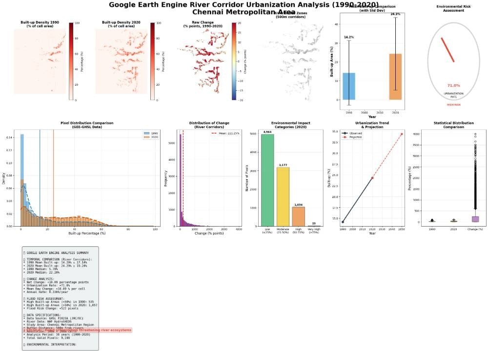
- comprehensive_analysis_dashboard.png - Multi-panel analytical figure
- spatial_distribution_maps.png - Built-up density spatial comparisons
- statistical_distributions.png - Histograms and KDE plots
- trend_projections.png - Future urbanization scenario plots
- environmental_risk_assessment.png - Risk gauge and impact visualizations
High-Level Steps
1. Geospatial Data Preparation
Initialize Earth Engine API, define AOI boundaries, configure output directories for data export2. River Corridor Delineation
Extract river networks from HydroSHEDS dataset, apply 500m buffer zones, export corridor geometries as vector data3. Built-up Surface Extraction
Acquire JRC/GHSL built-up datasets for target years (1990, 2020), clip to river corridors, normalize density values to percentages4. Temporal Change Computation
Calculate raw change metrics (2020-1990), derive percentage change rates, identify major development zones through threshold analysis5. Statistical Aggregation
Compute descriptive statistics (mean, median, standard deviation) for each temporal layer, mask NoData values, categorize environmental impact levels6. Multi-dimensional Visualization
Generate comprehensive analytical dashboard with spatial maps, temporal comparisons, statistical distributions, trend projections, and risk assessment gauges7. Environmental Impact Assessment
Synthesize quantitative metrics into urbanization rates, encroachment patterns, and future risk projections with detailed interpretative reporting🚀 Ready to implement this solution?
Access the complete code, step-by-step instructions, and interactive notebook in Nika Hub.
View Full Solution →