

Overview
NikaNotebook is a collaborative Python notebook environment designed specifically for geospatial data analysis. Built on Jupyter technology with real-time collaboration features, it enables teams to work together on spatial analysis projects with AI-powered assistance and seamless integration with Nika’s data ecosystem.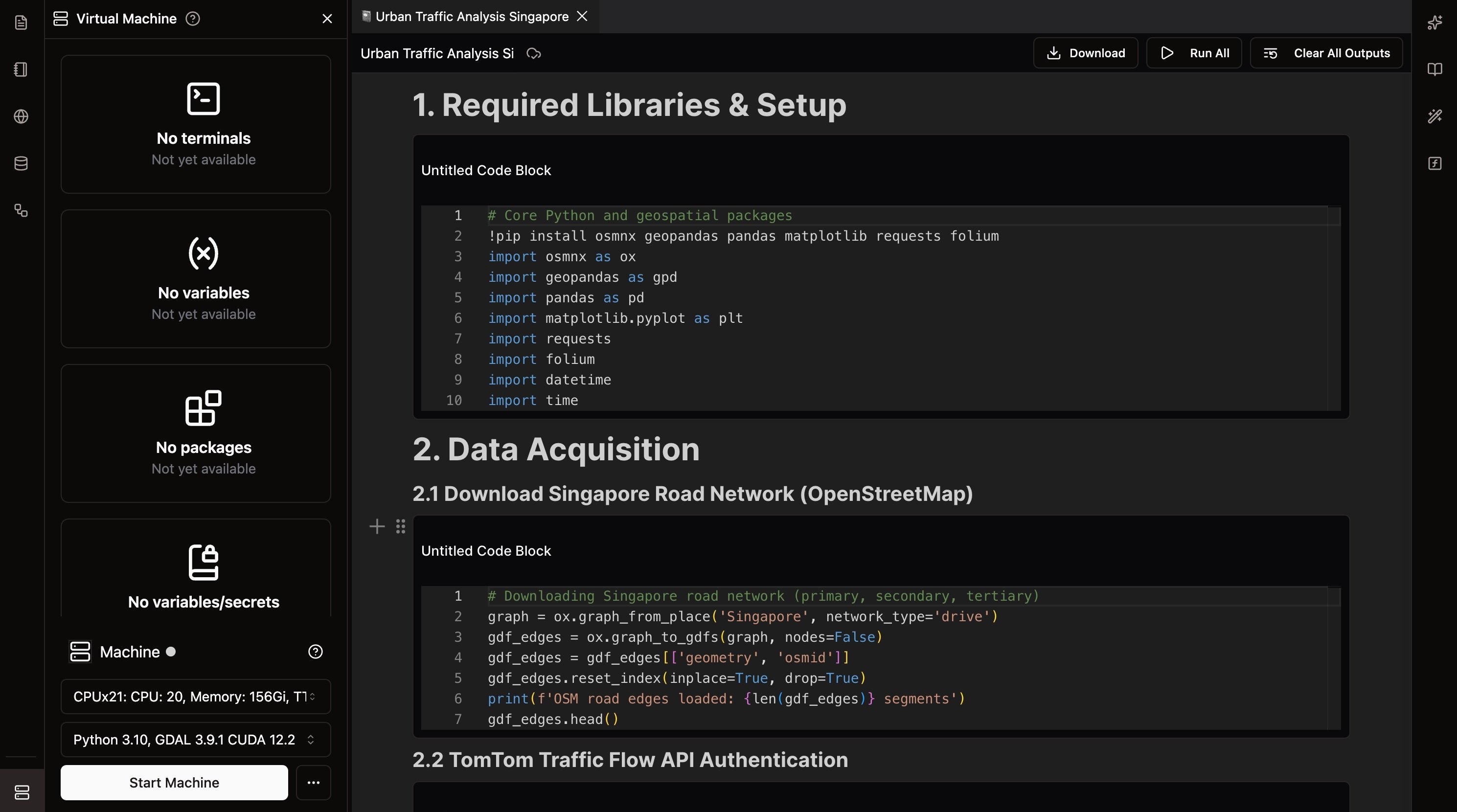
Key Features
Collaborative Notebooks
- Real-time Collaboration: Multiple users can edit notebooks simultaneously
- Live Cursor Tracking: See where team members are working in real-time
- Comment System: Add comments and discussions directly in notebooks
Geospatial-Focused Environment
- Pre-installed Libraries: GDAL, CUDA, Python, Linter
- Team preferred Libraries: Add a list of your usual library (to be built)
- Data Integration: Direct access to NikaWorkspace data lake
- AI Assistance: Get intelligent code modification suggestions from NikaGAIA
Server-Based Processings
- Offline Processing Enabled: Even if your internet is cut, your code that is running will run until completion on the server side and update the results for you to see when you reconnects back the next monitoring to continue your work
- Auto Shutoff Enabled: To save compute resources, the VM that is in idle state and no user is connected to it will auto shut off in 15 minutes
Flexible Compute Options
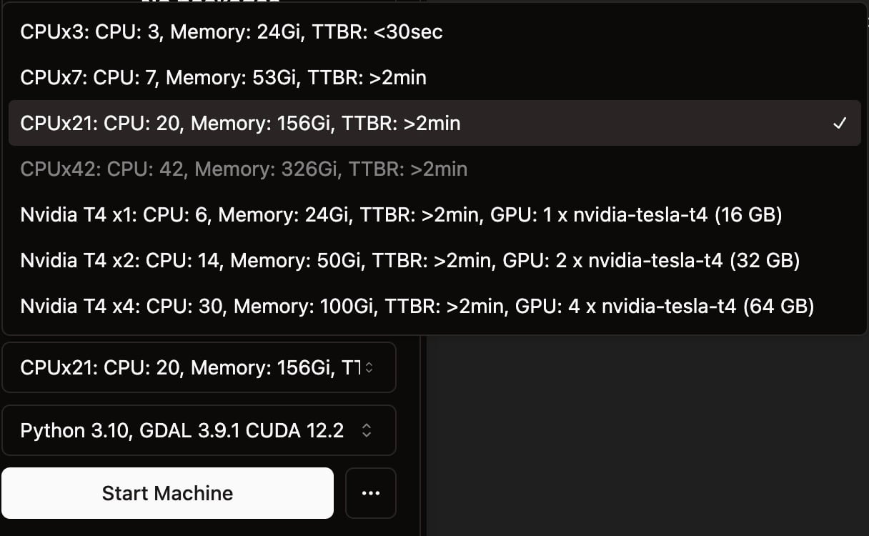
- CPU-Only VMs: High CPU-to-RAM ratio configurations (CPUx3: 3 cores/24GB, CPUx7: 7 cores/53GB, CPUx21: 20 cores/156GB, CPUx42: 42 cores/326GB) optimized for memory-heavy geospatial processing and large dataset analysis
- GPU-Enabled VMs: NVIDIA Tesla T4 configurations (T4x1: 6 cores/24GB/16GB GPU, T4x2: 14 cores/50GB/32GB GPU, T4x4: 30 cores/100GB/64GB GPU) designed for machine learning and AI workloads
- Custom Configurations: Even larger VMs with more RAM or H100 GPUs available upon request for enterprise-scale processing
Remote Cloud Execution
Run compute-heavy functions on dedicated VMs. Decorate any Python function with@run(compute=...), call .submit() to dispatch it to a separate runner pod, and keep working in the notebook while the job executes in parallel.
- Background execution and non-blocking: the notebook stays live while runs execute on their own machines, shutting down the VM does not cancel in-flight jobs
- Flexible compute per run: customize the run to use CPU-only or GPU-enabled VMs, independent of the notebook VM
- Results and logs: poll status, view logs, and retrieve results anytime after the run is completed
Output retention: Outputs from any run will only be kept for a maximum of
180 days. For reliability, write large files to
/data (your persistent
workspace storage) instead of returning them as run outputs.Monitoring Runs
Every run you submit with@run(...).submit() is tracked in the workspace, so you can follow its progress and read its logs in the UI.
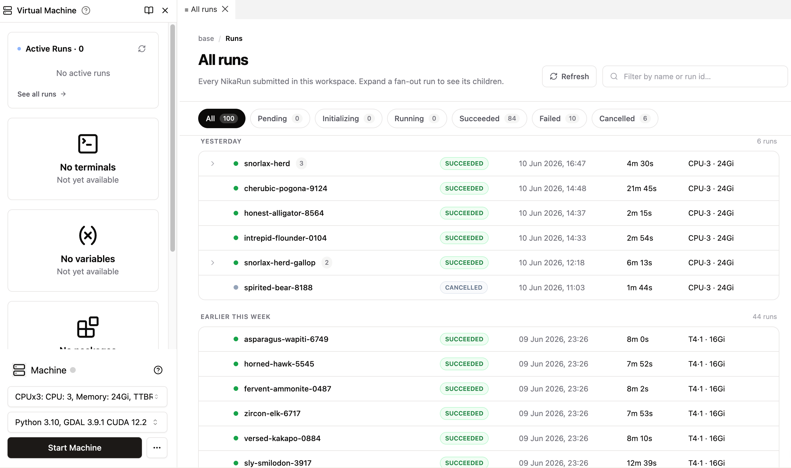
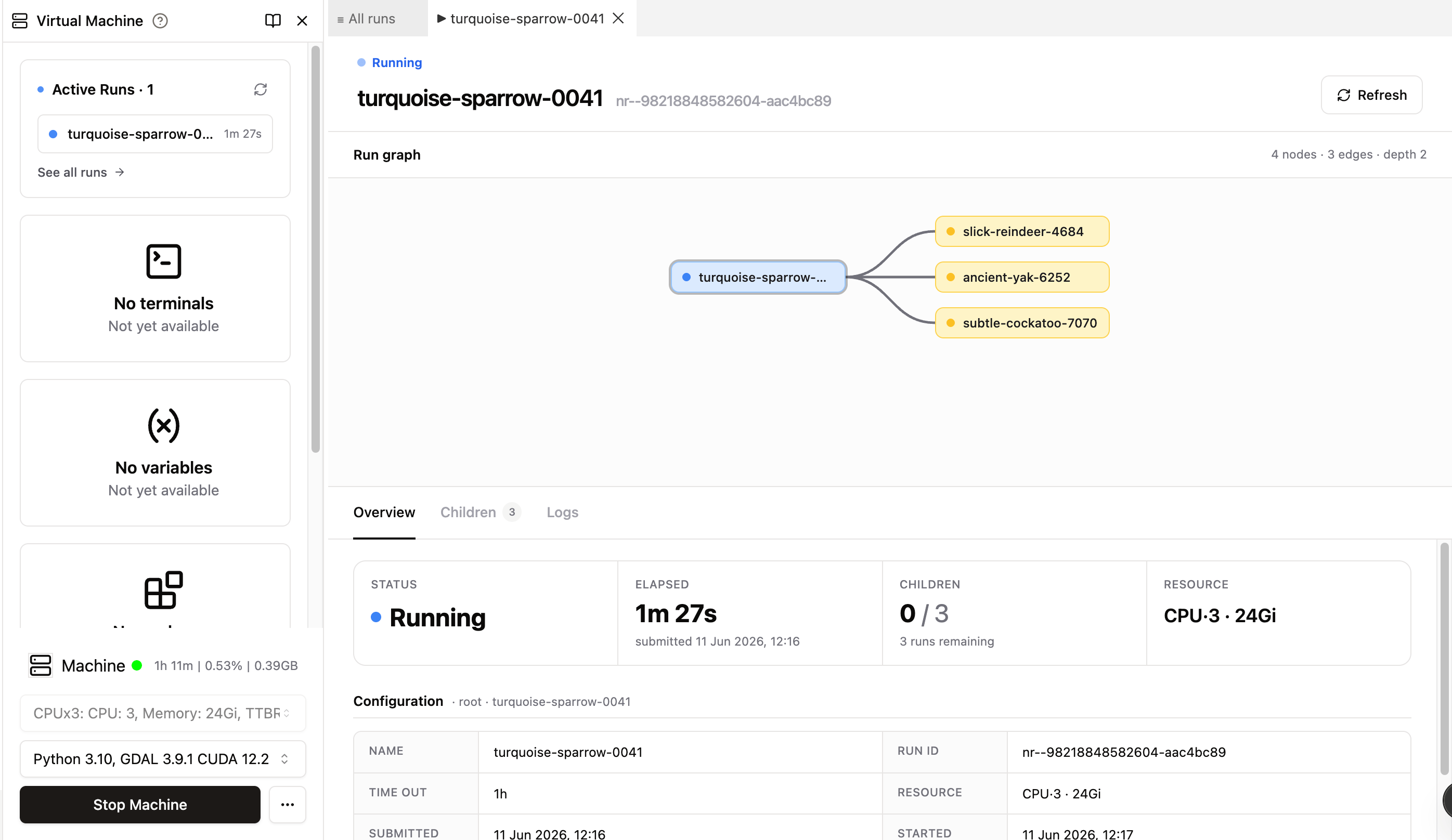
- Active Runs: a section at the top of the Virtual Machine side panel that lists runs still in progress, each with a status dot, name, status, and elapsed time. A run waiting on compute shows Queuing with the time left before its queue timeout. It refreshes automatically; See all runs opens the full list.
-
All Runs: every run submitted in the workspace, grouped by time and filterable by status (Pending, Queuing, Initializing, Running, Succeeded, Failed, Cancelled). Search by name or run ID, and expand a fan-out run to see its children.
-
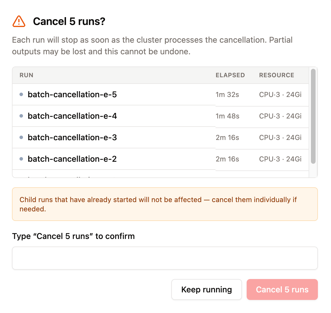
Cancel runs in bulk: tick the checkbox on any active runs in the All Runs list — a floating bar shows how many are selected, with Clear and a Cancel N runs action. Confirm in the dialog by typing the highlighted phrase. Cancellation is requested for each selected run and can’t be undone, so in-progress work may be lost; child runs that have already started are not affected and can be cancelled individually.
-
Run Detail: opens from any run. A fan-out run graph shows the run tree (a parent run and its child runs), and Overview, Children, Logs, and Metrics tabs cover the run’s status, configuration (name, run ID, resource, queue timeout, run/execution timeout, and submitted, started, finished and duration times), child runs, logs, and resource usage.
-
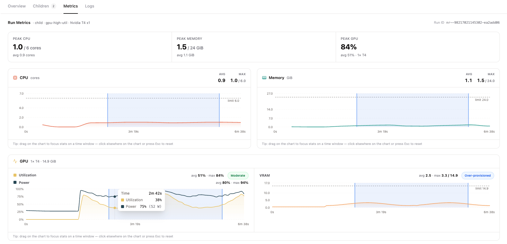
Metrics tab: for completed runs, see CPU, memory, and (when the machine has one) GPU utilisation, VRAM, and power draw sampled across the run. Peak headline cards summarise the run at a glance, and each chart carries a fit verdict — Well-utilised, Right-sized, Over-provisioned, Near limit, OOM risk — so it’s obvious whether the machine size matched the workload.
- Focus stats on a time window: drag on any chart to highlight a range. Averages, peaks and verdicts recompute for just that window — useful for excluding warm-up, setup, or a spike you want to inspect. Click elsewhere on the chart or press Esc to clear the selection and return to full-run stats.
- Focus stats on a time window: drag on any chart to highlight a range. Averages, peaks and verdicts recompute for just that window — useful for excluding warm-up, setup, or a spike you want to inspect. Click elsewhere on the chart or press Esc to clear the selection and return to full-run stats.