
Overview

NikaNotebook is a collaborative Python notebook environment designed specifically for geospatial data analysis. Built on Jupyter technology with real-time collaboration features, it enables teams to work together on spatial analysis projects with AI-powered assistance and seamless integration with Nika’s data ecosystem.
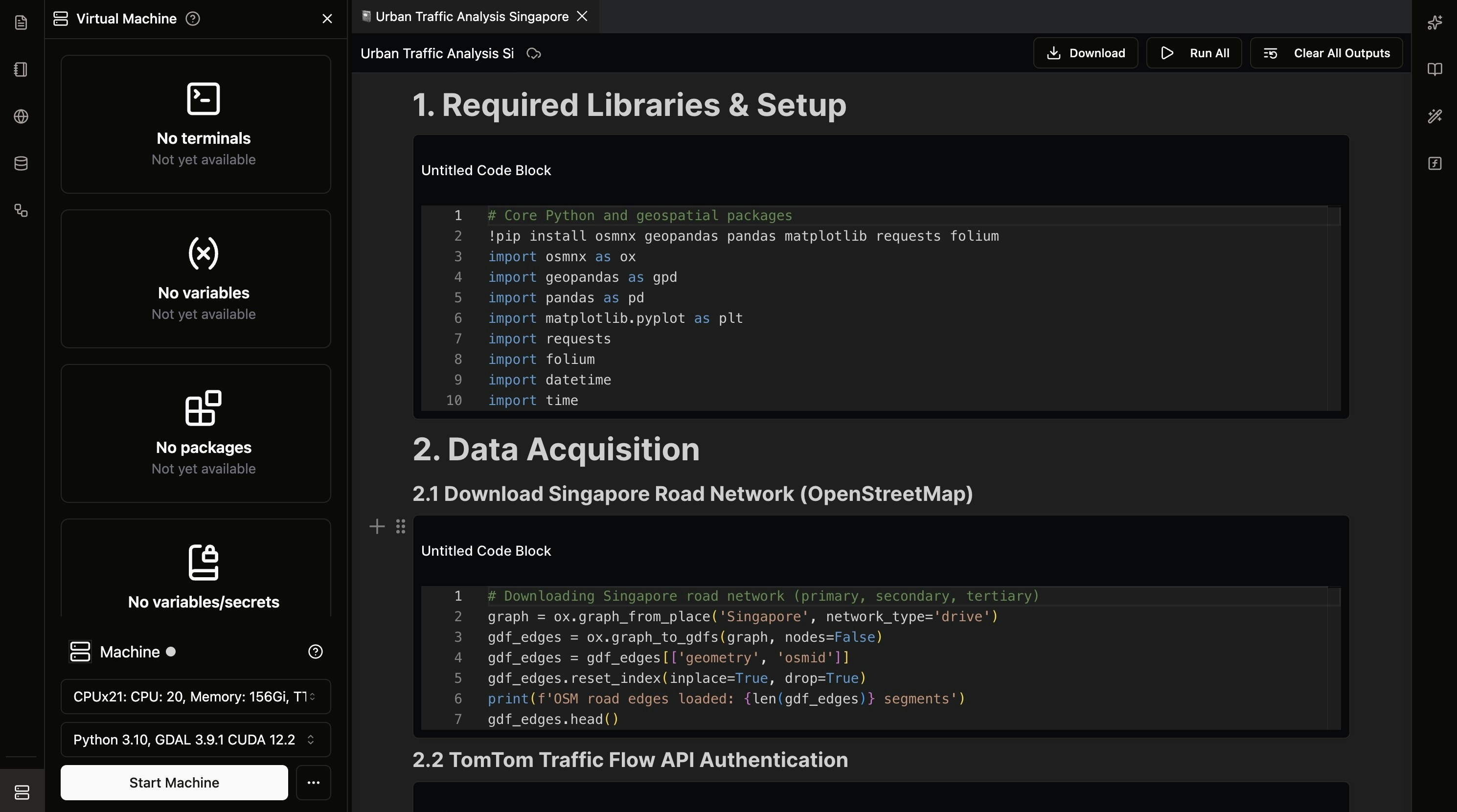
 NikaNotebook Interface

Key Features

Collaborative Notebooks

  • Real-time Collaboration: Multiple users can edit notebooks simultaneously
  • Live Cursor Tracking: See where team members are working in real-time
  • Comment System: Add comments and discussions directly in notebooks

Geospatial-Focused Environment

  • Pre-installed Libraries: GDAL, CUDA, Python, Linter
  • Team preferred Libraries: Add a list of your usual library (to be built)
  • Data Integration: Direct access to NikaWorkspace data lake
  • AI Assistance: Get intelligent code modification suggestions from NikaGAIA

Server-Based Processings

  • Offline Processing Enabled: Even if your internet is cut, your code that is running will run until completion on the server side and update the results for you to see when you reconnects back the next monitoring to continue your work
  • Auto Shutoff Enabled: To save compute resources, the VM that is in idle state and no user is connected to it will auto shut off in 15 minutes

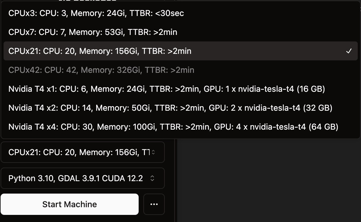
Flexible Compute Options

  • CPU-Only VMs: High CPU-to-RAM ratio configurations (CPUx3: 3 cores/24GB, CPUx7: 7 cores/53GB, CPUx21: 20 cores/156GB, CPUx42: 42 cores/326GB) optimized for memory-heavy geospatial processing and large dataset analysis
  • GPU-Enabled VMs: NVIDIA Tesla T4 configurations (T4x1: 6 cores/24GB/16GB GPU, T4x2: 14 cores/50GB/32GB GPU, T4x4: 30 cores/100GB/64GB GPU) designed for machine learning and AI workloads
  • Custom Configurations: Even larger VMs with more RAM or H100 GPUs available upon request for enterprise-scale processing
NikaNotebook Interface

Python Notebook Examples in NikaNotebook

Spatial Analysis

import geopandas as gpd
import pandas as pd
from shapely.geometry import Point, Polygon
from shapely.ops import voronoi_diagram
import folium

# Buffer analysis - Create 1km buffers around points
points_gdf = gpd.read_file('points.geojson')
buffers = points_gdf.geometry.buffer(1000)  # 1000 meters

# Intersection operations - Find overlapping areas
layer1 = gpd.read_file('layer1.geojson')
layer2 = gpd.read_file('layer2.geojson')
overlaps = gpd.overlay(layer1, layer2, how='intersection')

# Distance calculations - Calculate distances between features
points = gpd.read_file('points.geojson')
polygons = gpd.read_file('polygons.geojson')
distances = points.geometry.apply(lambda x: polygons.geometry.distance(x).min())

# Spatial joins - Join attributes based on location
joined = gpd.sjoin(points, polygons, how='left', predicate='within')

# Voronoi diagrams - Create service areas
from scipy.spatial import Voronoi
import numpy as np
coords = np.array([[p.x, p.y] for p in points.geometry])
voronoi = Voronoi(coords)

Statistical Analysis

import numpy as np
from scipy import stats
import pandas as pd
from libpysal.weights import Queen
from esda.moran import Moran

# Descriptive statistics for spatial data
stats = spatial_data[['population', 'area']].describe()

# Spatial autocorrelation - Moran's I test
w = Queen.from_dataframe(spatial_data)
morans_i = Moran(spatial_data['value'], w)

# Hot spot analysis - Getis-Ord Gi* statistic
from esda.getisord import G_Local
g_local = G_Local(spatial_data['crime_rate'], w)
hotspots = spatial_data[g_local.p_sim < 0.05]

# Regression analysis with spatial variables
from sklearn.linear_model import LinearRegression
X = spatial_data[['distance_to_center', 'area']]
y = spatial_data['price']
model = LinearRegression().fit(X, y)

Machine Learning

from sklearn.cluster import KMeans
from sklearn.ensemble import RandomForestClassifier
from sklearn.preprocessing import StandardScaler
import pandas as pd

# Spatial clustering - Group similar locations
coords = spatial_data[['longitude', 'latitude']].values
kmeans = KMeans(n_clusters=5, random_state=42)
clusters = kmeans.fit_predict(coords)

# Classification - Predict land use from satellite imagery
X = raster_data.reshape(-1, raster_data.shape[-1])
y = training_points['land_use']
rf = RandomForestClassifier(n_estimators=100, random_state=42)
rf.fit(X, y)
land_use_pred = rf.predict(X)

# Time series analysis - Analyze temporal patterns
data['date'] = pd.to_datetime(data['date'])
monthly_trends = data.groupby(data['date'].dt.to_period('M'))['temperature'].mean()

# Anomaly detection - Find unusual spatial patterns
from sklearn.ensemble import IsolationForest
iso_forest = IsolationForest(contamination=0.1, random_state=42)
anomalies = iso_forest.fit_predict(spatial_data[['value1', 'value2']])
There are more real-life examples published by Nika community at https://planet.nika.eco/en/hub/notebooks

Getting Started

Learn how to perform geospatial analysis with NikaNotebook in 7 easy steps. This comprehensive tutorial will guide you from creating your first notebook to publishing your analysis results. Start the Geospatial Analysis Tutorial →

Get Expert Help